Functional hash tables explained

Prologue: The quest for a functional hash table for Goblins

For those of us that use the Lisp family of programming languages, we have much appreciation for the humble pair. Using pairs, we can construct singly-linked lists and key/value mappings called association lists. Lists built from pairs have the pleasant property of being immutable (if you abstain from using setters!) and persistent: extending a list with a new element creates a new list that shares all the data from the original list. Adding to a list is a constant time operation, but lookup is linear time. Thus, lists are not appropriate when we need constant time lookup. For that, we need hash tables.

The classic hash table is a mutable data structure and one that our Lisp of choice (Guile, a Scheme implementation) includes in its standard library, like most languages. Hash tables are neither immutable nor persistent; adding or removing a new key/value pair to/from a hash table performs an in-place modification of the underlying memory. Mutable data structures introduce an entire class of bug possibilities that immutable data structures avoid, and they’re particularly tricky to use successfully in a multi-threaded program.

Fortunately, there exists an immutable, persistent data structure that is suitable: the Hash Array Mapped Trie or HAMT, for short. This data structure was introduced by Phil Bagwell in the paper “Ideal Hash Trees” (2001). HAMTs were popularized in the Lisp world by Clojure over a decade ago. Unfortunately, Guile does not currently provide a HAMT-based functional hash table in its standard library.

Instead, Guile comes with the VList, another one of Phil Bagwell’s creations which can be used to build a VHash. Goblins currently uses VLists for its functional hash table needs, but HAMTs are better suited for the task.

There are various implementations of HAMTs in Scheme floating about, but none of them seem to have notable adoption in a major Guile project. So, we thought we’d write our own that we could ensure meets the needs of Goblins, compiles on Hoot, and that might just be useful enough to send upstream for inclusion into Guile after it’s been battle tested. To that end, we recently added the (goblins utils hashmap) module. This will become the base for a future re-implementation of the ^ghash actor.

Okay, enough context. Let’s talk about HAMTs!

What the hoot is a HAMT anyway?

From the outside, HAMTs can seem rather mysterious and intimidating. That’s how I felt about them, at least. However, once I dug into the topic and started writing some code, I was pleasantly surprised that the essential details were not too complicated.

As mentioned previously, the HAMT is an immutable, persistent data structure that associates keys with their respective values, just like a regular hash table. By utilizing a special kind of tree known as a “trie” plus some nifty bit shifting tricks, HAMTs achieve effectively constant time insertion, deletion, and lookup despite all operations being logarithmic time on paper.

A trie differs from a tree in the following way: tries only store keys in their leaf nodes. If you’re familiar with binary search trees, tries aren’t like that. Instead, the key itself (or the hash thereof, in our case) encodes the path through the trie to the appropriate leaf node containing the associated value. Tries are also called “prefix trees” for this reason.

A binary tree node can have at most two children, but HAMTs have a much larger branching factor (typically 32). These tries are wide and shallow, so few nodes need to be traversed to find the value for any given key. This is why the logarithmic time complexity of HAMT operations can be treated as if it were constant time in practice.

Trie representation

To explain, let’s start by defining a trie node using a branching factor of 32. At its simplest, we can think of a trie node as a 32-element array. Each element of the trie can contain either a leaf node (a key/value pair) or a pointer to a subtrie (another 32 element array).

For example, a HAMT with 3 entries might look like this:

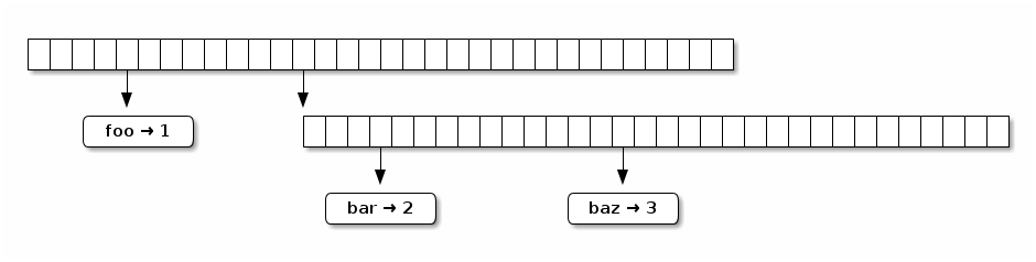
This is nice and simple, but it’s a little too simple. With such a large branching factor, it’s likely that many boxes in the trie will have nothing in them, like in the above example. This is a waste of space. The issue is further compounded by immutability: adding or removing a single element requires allocating a new 32 element array. For the sake of efficiency, we need to do better.

Instead, we’ll use a sparse array that only stores the occupied elements of the trie node. To keep track of which elements of the theoretical 32 element array are occupied, we’ll use a bitmap. Below is an example trie:

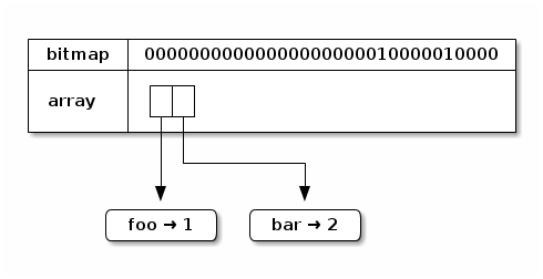
In the above example, bits 4 and 10 (starting from the right) are set. This means that of the 32 possible elements, only 2 are currently occupied. Thus, the size of the underlying array is 2.

To get the number of occupied elements in the trie node, we simply count the number of 1s in the bitmap. This is known as the “population count”. (We could also just check the size of the array, but this bit counting idea is about to have another important use.)

To retrieve the value at index 10, we need to perform a translation to get an index into the underlying array. To do this, we compute the population count of the bits set to the right of bit 10. There is 1 bit set: bit 4. Thus, the value we’re looking for is stored at index 1 in the underlying array. If we take a peek, we find bar → 2 there.

Thanks to this sparse storage technique, insertion/deletion operations will allocate less memory overall.

Insertion algorithm

With the trie representation out of the way, let’s walk through the algorithm to insert a new key/value pair. The insertion algorithm covers all the essential aspects of working with a HAMT.

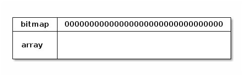
Let’s say we want insert the mapping foo→42 into an empty HAMT. The empty HAMT consists of a single node with an empty bitmap and an empty array:

To figure out where to store the key foo, we first need to compute the hash code for it. For ease of demonstration, we’ll use 10-bit hash codes. (In practice, 32 bits or more is ideal.)

Let’s say our fictitious hash function produces the hash bits 1000010001 for foo.

Each trie node has 32 possible branches. Thus, the range of indices for a node can be represented using a 5-bit unsigned integer. What if we took the 5 most significant bits of the hash code and used that as our index into the trie? Wow, that sounds like a clever idea! Let’s do that!

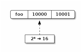
So, foo gets inserted at index 16. The original trie is empty, so we’ll make a new trie with a single leaf node. To do this, we need to set bit 16 in our bitmap and create an array with just one key/value pair in it. Our output trie looks like this:

Note that we only examined 5 bits of the hash code. We only need to examine as many bits in the hash as it takes to find an empty element.

Let’s insert another key/value pair, this time for key bar and value 17. Our made-up hash code for bar is 0100100001. Repeating the process above, the most significant 5 bits are 01001, so our index is 9, another unoccupied index. Our new trie looks like this:

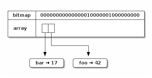
Because 9 < 16, the entry for bar is stored in array index 0, followed by foo.

As a last example, let’s insert a key/value pair where the most significant bits of the hash code collide with an existing entry. This time, the key is baz and the value is 66. Our made-up hash code for baz is 1000000001.

The most significant 5 bits are 10000, so our index is 16. Now things get interesting because 16 is already occupied; the first 5 bits are not enough to distinguish between the keys foo and baz! To resolve this, we’ll replace the leaf node with a subtrie that uses the next 5 bits when calculating indices. The resulting root trie node will look sort of like this:

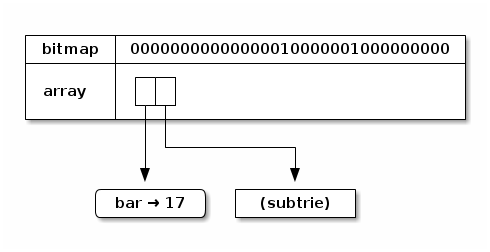
In the figure above, subtrie is a placeholder for the new trie we need to construct to hold the mappings for foo and baz.

To create the subtrie, we just recursively apply the same algorithm we’ve already been using but with different bits. Now we’re looking at these the least significant 5 bits of the hash codes:

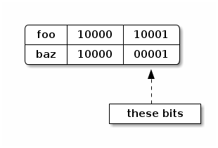
The index for foo is 17, and the index for baz is 1. So, our new subtrie will have bits 1 and 17 set, and contain 2 leaf nodes:

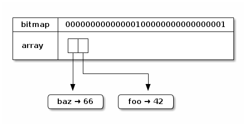
Putting it all together, the complete trie looks like this:

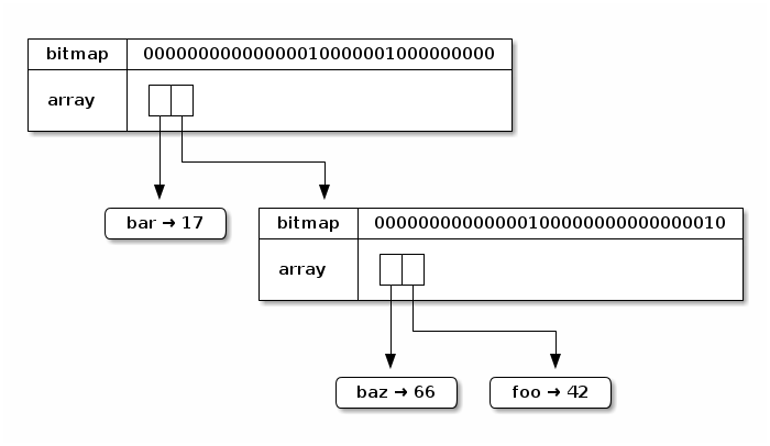
Each insertion creates a new trie. The new trie shares nearly all of the data with the original trie. Only the root node and the visited subtries need to be allocated afresh. This makes insertion even into large HAMTs quite efficient.

The partial hash collision described above could happen recursively, in which case the trie will grow yet another level deeper upon each iteration. The worst case scenario is that two or more keys have the same exact hash code. A good hash function and lots of hash bits will make this a very rare occurrence, and a robust insertion algorithm needs to account for this case. We’ll gloss over this edge case here, but hash collisions can be handled by “bottoming out” to a special leaf node: a linked list of the colliding key/value pairs. These lists need to be traversed linearly when necessary upon lookup or future insertions that cause more collisions. In practice, these collision lists tend to be quite short, often only of length 2.

Wrapping up

The insertion algorithm explains all of the essential elements of a HAMT and how to work with its sparse storage structure, but we’ll touch upon lookup and deletion very briefly.

Looking up the value for a key follows the same basic process as insertion, but in a read-only manner. If the hash bits point to an unoccupied element of a trie node then the search fails right then and there. If the bits point to a leaf node with a matching key, the search succeeds. If the key doesn’t match, the search fails. Finally, if the bits point to a subtrie, we recursively search that subtrie with the next set of bits.

Deletion is the most complicated operation as it involves path compression when subtries become empty. If you’ve been successfully nerd sniped by this blog post then consider this a homework assignment. Give Phil Bagwell’s paper a read! 🙂

Thanks for following along! Hope this was fun!